| Version 3 (modified by , 12 years ago) ( diff ) |
|---|
Subsets in Petascope
In this page we will describe how subsets (trims and slices) are treated by Petascope. Before this you will have to understand how the topology of a grid coverage is interpreted with regards to its origin, its bounding-box and the assumptions on the sample space. Some practical example will then be proposed.
Geometric interpretation of a coverage
This section will focus on how the topology of a grid coverage is stored in the metadata database and how Petascope interprets it. For point-clouds (multipoint coverages, in the GML realm), the subject is straightforward: each point is a 0D element (please not that bbox description of point-clouds are currently not implemented: see #571).
When it comes to the so-called domainSet of a coverage (hereby also called domain, topology or geometry), the metadata database (petascopedb) follows pretty much the GML model for rectified grids: the grid origin and one offset vector per grid axis are enough to deduce the full domainSet of such (regular) grids. When it comes to referenceable grids, the domainSet still is kept in a compact vectorial form by adding weighting coefficients to one or more offset vectors. For more on this please refer to the [PetascopeUserGuide user guide].
- What is a grid?
- As by GML standard a grid is a network composed of two or more sets of curves in which the members of each set intersect the members of the other sets in an algorithmic way. The intersections of the curves are represented by points: a point is 0D and is defined by a single coordinate tuple and implements ISO:19107
GM_Point(see D.2.3.3 and ISO 19107:2003, 6.3.11).
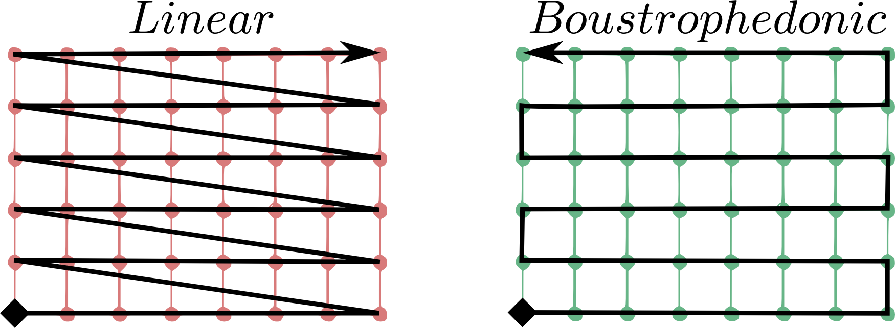
A first question arises on where to put the grid origin. The GMLCOV standard says that the mapping from the domain to the range (feature space, payload, values) of a coverage is specified through a function, formally a gml:coverageFunction. We do not currently support the configuration of such function, whereas we stick to the default mapping which is indeed assumed when no coverage function is described. From the GML standard: If the gml:coverageFunction property is omitted for a gridded coverage (including rectified gridded coverages) the gml:startPoint is assumed to be the value of the gml:low property in the gml:Grid geometry, and the gml:sequenceRule is assumed to be linear and the gml:axisOrder property is assumed to be +1 +2.
To better understand this, the following image is showing the difference between a linear sequence rule (what we adopt) and an other kind of mapping, the so-called boustrophedonic this page for other available rules:

In the imag, it is assumed that the first grid axis (+1) is the horizontal axis, while the second (+2) is the vertical axis; the grid starting point is the full diamond.
Sticking to the linear sequence rule was the best choice for rasdaman since that is the same rule which rasdaman itself uses to print the values of cells in an collection/marray.
Coming back to the origin question on where to put the origin of our grid coverages, we have to make it coincide to what the starting value represents in rasdaman, the marray origin.
As often done in GIS applications, the origin of an image is set to be its upper-left corner: this finally means that the origin of our rectified and referenceable grid coverages shall be there too in order to provide a coherent GML/GMLCOV coverage, where the domain is really mapped to the range of the coverage with the default coverage function. Note that placing the origin in the upper-left corner of an image means that the offset vector along the northing axis will point South, hence will have negative norm (in case the direction of the CRS axis points North!).
When it comes to further dimensions (a third elevation axis, time, etc.), the position of the origin depends on the way data has been ingested. Taking the example of a time series, if the marray origin (which we can denote as [0:0:__:0], though it is more precisely described as [dom.lo[0]:dom.lo[1]:__:dom.lo[n]) is the earliest moment in time, then the grid origin will be the easliest moment in the series, and the offset vector in time will point to the future (positive norm); in the other case, the origin will be the latest time in the series, and its vector will point to the past (negative norm).
To summarize, in any case the grid origin must point to the marray origin. This is important in order to properly implement our linear sequence rule.
A second question arises on how to treat coverage points: are they points or are they areas? The formal ISO term for the area of a point is sample space. We will refer to it as well as footprint or area. The GML standard provides guidance on the way to interpret a coverage: "When a grid point is used to represent a sample space (e.g. image pixel), the grid point represents the center of the sample space (see ISO 19123:2005, 8.2.2)".
In spite of this, there is no formal way to describe GML-wise the footprint of the points of a grid. While the configuration of sample spaces is still just on the wishlist (see #680), our current policy applies distinct choices separately for each grid axis, in the following way:
- regular axis: when a grid axis as equal spacing between each of its points, then it is assumed that the sample space of the points is equal to this spacing (resolution) and that the grid points are in the middle of this interval;
- irregular axis: when a grid axis as an uneven spacing between its points, then there is no (currently implemented) way to either express or deduce its sample space, hence 0D points are assumed here (no footprint).
Such policy translated in practice to a point-is-pixel-center interpretation of regular rectified images. The following art explains it visually:
  KEY
          # = grid origin             o = pixel corners
          + = grid points             @ = upper-left corner of BBOX
  {v_0,v_1} = offset vectors

  |======== GRID COVERAGE MODEL =========|    |===== GRID COVERAGE + FOOTPRINTS =====|

                                             {UL}
           v_0                                 @-------o-------o-------o-------o--- -
       -------->                               |       |       |       |       |
     . #-------+-------+-------+--- -          |   #   |   +   |   +   |   +   |
 v_1 | |       |       |       |               |       |       |       |       |
     | |       |       |       .               o-------o-------o-------o-------o-- -
     V |       |       |       .               |       |       |       |       .
       +-------+-------+--- -                  |   +   |   +   |   +   |       .
       |       |       |                       |       |       |       |
       |       |       .                       o-------o-------o-------o-- -
       |       |       .                       |       |       |       .
       +-------+--- -                          |   +   |   +   .       .
       |       |                               |       |       .
       |       .                               o-------o--- -
       |       .                               |       .
       +--- -                                  .   +   .
       .                                       .
       .

  |======================================|    |======================================|
The left-side grid is the GML coverage model for a regular grid: it is a network of (rectilinear) curves, whose intersections determine the grid points '+'. The description of this model is what petascopedb knows about the grid.
The right-hand grid is instead how Petascope inteprests the information in petascopedb, and hence is the coverage that is seen by the enduser. You can see that, being this a regular grid, sample spaces (pixels) are added in the preception of the coverage, causing an extension of the bbox (gml:boundedBy) of half-pixel on all sides. The width of the pixel is assumed to be equal to the (regular) spacing of the grid points, hence each pixel is of size |v_0| x |v_1|, being |*| the norm operator.
As a final example, imagine that we take this regular 2D pattern and we build a series of such images on irregular levels of altitude:
  KEY
          # = grid origin             X = ticks of the CRS height axis
          + = grid points             O = origin of the CRS height axis
  {v_0,v_2} = offset vectors


      O-------X--------X----------------------------X----------X-----X-----------> height
      |
      |       ---> v_2
      |     . #________+____________________________+__________+_____+
      | v_0 | |        |                            |          |     |
      |     V +________+____________________________+__________+_____+
      |       |        |                            |          |     |
      |       +________+____________________________+__________+_____+
      |       |        |                            |          |     |
      |       +________+____________________________+__________+_____+
      |       |        |                            |          |     |
      V       .        .                            .          .     .
   easting
In petascopedb we will need to add an other axis to the coverage topology, assigning a vector to it, v_2 (we support gmlrgrid:ReferenceableGridByVectors only, hence each axis of any kind of grid will have a vector). Weighting coefficients will then determine the height of each new z-level of the cube: such heights are encoded as distance from the grid origin '#' normalized by the offset vector v_2. Please note that the vector of northings v_1 is not visible due to perspective: the image is showing the XZ plane.
Regarding the sample spaces, while Petascope will still assume the points are pixels on the XY plane (eastings/northings), it will instead assume 0D footprint along Z, that is along height: this means that the extent of the cube along height will exactly fit to the lowest and highest layers, and that input Z slices will have to select the exact value of an existing layer.
The latter wouls not hold on regular axes: this is because input subsets are targeting the sample spaces, and not just the grid points, but this is covered more deeply in the following section.
input and output subsetting
..open/closed intervals (we have closed now: reply to this post in our mailing list to discuss this topic), output subsets (expressed via gml:Envelope) fit to mimimum bounding box: reduced area until is greater than a unit = pixel size.
In general, pixel validity is meant as half open [min,max), whereas the subsets are meant as closed intervals [a,b].
Subsets with extent smaller than a pixel resolution return the pixel(s) that include(s) it.
Examples
This is probably better understood by means of examples:
--------------------
mean_summer_airtemp (EPSG:4326)
[0:885, 0:710]
x(111.975, 156.275)
y(-44.525, -8.975)
res(0.05, 0.05)
--------------------

   130.975  131.025  131.075  131.125  131.175
X:  ...o--------o--------o--------o--------o...
         cell380  cell381  cell382  cell383
          [s1]
       [== s2 ==]
         [==== s3 ====]
         [======== s4 =======]
    [=================== s5 ===================] (BEYOND BBOX)

    -22.975  -22.925  -22.875  -22.825  -22.795
Y:  ...o--------o--------o--------o--------o...
         cell280  cell279  cell278  cell277
          [s1]
       [== s2 ==]
         [==== s3 ====]
         [======== s4 =======]
    [=================== s5 ===================] (BEYOND BBOX)

s1: m[380:380, 280:280]
 - for m in (mean_summer_airtemp) return encode(trim(m, {x(131:131.01), y(-22.951:-22.95)}),"csv")
 - http://localhost:8080/petascope/wcs2?
      service=WCS&version=2.0.0&request=GetCoverage&coverageid=mean_summer_airtemp&
      subset=x(131,131.01)&subset=y(-22.951,-22.95)

s2: m[380:381, 279:280]
 - for m in (mean_summer_airtemp) return encode(trim(m, {x(130.975:131.025), y(-22.975:-22.925)}),"csv")
 - http://localhost:8080/petascope/wcs2?
      service=WCS&version=2.0.0&request=GetCoverage&coverageid=mean_summer_airtemp&
      subset=x(130.975,131.025)&subset=y(-22.975,-22.925)

s3: m[380:381, 279:280]
 - for m in (mean_summer_airtemp) return encode(trim(m, {x(131:131.05), y(-22.95:-22.9)}),"csv")
 - http://localhost:8080/petascope/wcs2?
      service=WCS&version=2.0.0&request=GetCoverage&coverageid=mean_summer_airtemp&
      subset=x(131,131.05)&subset=y(-22.95,-22.9)

s4: m[380:382, 278:280]
 - for m in (mean_summer_airtemp) return encode(trim(m, {x(131:131.1), y(-22.95:-22.85)}),"csv")
 - http://localhost:8080/petascope/wcs2?
      service=WCS&version=2.0.0&request=GetCoverage&coverageid=mean_summer_airtemp&
      subset=x(131,131.1)&subset=y(-22.95,-22.85)

s5: m[0:885, 0:710]
 - for m in (mean_summer_airtemp) return encode(trim(m, {x(100:200), y(-50:50)}),"csv")
 - http://localhost:8080/petascope/wcs2?
      service=WCS&version=2.0.0&request=GetCoverage&coverageid=mean_summer_airtemp&
      subset=x(100,200)&subset=y(-50,50)

-=-=-=-=-=-=-=-=-=-=-=-=-=-=-=-=-=-=-=-=-=-=-=-=-=-=-=-=-=-=-=-=-=-=-=

TIME AXIS EXAMPLE:

     09h20    10h20    11h20    12h20    13h20
T:     o--------o--------o--------o--------o
          cell0    cell1    cell2    cell3
          [s1]
       [== s2 ==]
         [==== s3 ====]
         [======== s4 =======]
    [=================== s5 ===================]

------------------------------------------------------------------------------------------------
s1: (9h25,9h30) --> [LOx:HIx, LOy:HIy, 0:0]
 - http://localhost:8080/petascope/wcs2?
     service=WCS&version=2.0.0&request=GetCoverage&coverageid=MODIS_33N_2010170_WGS84&
     subset=x(10,11)&subset=y(45,46)&subset=t(2010-06-19T09:25,2010-06-19T09:30)
 - for c in (MODIS_33N_2010170_WGS84) return encode(
    trim(
      c,{t:"http://www.opengis.net/def/crs/ISO/0/8601"                        ("2010-06-19T09:25":"2010-06-19T09:30"),
         y:"http://kahlua.eecs.jacobs-university.de:8080/def/crs/EPSG/0/4326" (45:46),
         x:"http://kahlua.eecs.jacobs-university.de:8080/def/crs/EPSG/0/4326" (10:11)}),
  "csv")
------------------------------------------------------------------------------------------------
s2: (9h20,10h20) --> [LOx:HIx, LOy:HIy, 0:1]
 - http://localhost:8080/petascope/wcs2?
      service=WCS&version=2.0.0&request=GetCoverage&coverageid=MODIS_33N_2010170_WGS84&
      subset=x(10,11)&subset=y(45,46)&subset=t(2010-06-19T09:20,2010-06-19T10:20)
 - for c in (MODIS_33N_2010170_WGS84) return encode(
    trim(
      c,{t:"http://www.opengis.net/def/crs/ISO/0/8601"                        ("2010-06-19T09:20":"2010-06-19T10:20"),
         y:"http://kahlua.eecs.jacobs-university.de:8080/def/crs/EPSG/0/4326" (45:46),
         x:"http://kahlua.eecs.jacobs-university.de:8080/def/crs/EPSG/0/4326" (10:11)}),
  "csv")
------------------------------------------------------------------------------------------------
s3: (10h00,11h00) --> [LOx:HIx, LOy:HIy, 0:1]
 - http://localhost:8080/petascope/wcs2?
      service=WCS&version=2.0.0&request=GetCoverage&coverageid=MODIS_33N_2010170_WGS84&
      subset=x(10,11)&subset=y(45,46)&subset=t(2010-06-19T10:00,2010-06-19T11:00)
 - for c in (MODIS_33N_2010170_WGS84) return encode(
    trim(
      c,{t:"http://www.opengis.net/def/crs/ISO/0/8601"                        ("2010-06-19T10:00":"2010-06-19T11:00"),
         y:"http://kahlua.eecs.jacobs-university.de:8080/def/crs/EPSG/0/4326" (45:46),
         x:"http://kahlua.eecs.jacobs-university.de:8080/def/crs/EPSG/0/4326" (10:11)}),
  "csv")
------------------------------------------------------------------------------------------------
s4: (9h30,11h50) --> [LOx:HIx, LOy:HIy, 0:2]
 - http://localhost:8080/petascope/wcs2?
      service=WCS&version=2.0.0&request=GetCoverage&coverageid=MODIS_33N_2010170_WGS84&
      subset=x(10,11)&subset=y(45,46)&subset=t(2010-06-19T09:30,2010-06-19T11:50)
 - for c in (MODIS_33N_2010170_WGS84) return encode(
    trim(
      c,{t:"http://www.opengis.net/def/crs/ISO/0/8601"                        ("2010-06-19T09:30":"2010-06-19T11:50"),
         y:"http://kahlua.eecs.jacobs-university.de:8080/def/crs/EPSG/0/4326" (45:46),
         x:"http://kahlua.eecs.jacobs-university.de:8080/def/crs/EPSG/0/4326" (10:11)}),
  "csv")
------------------------------------------------------------------------------------------------
s5: (9h00,14h00) --> [LOx:HIx, LOy:HIy, 0:3]
 - http://localhost:8080/petascope/wcs2?
      service=WCS&version=2.0.0&request=GetCoverage&coverageid=MODIS_33N_2010170_WGS84&
      subset=x(10,11)&subset=y(45,46)&subset=t(2010-06-19T09:00,2010-06-19T14:00)
 - for c in (MODIS_33N_2010170_WGS84) return encode(
    trim(
      c,{t:"http://www.opengis.net/def/crs/ISO/0/8601"                        ("2010-06-19T09:00":"2010-06-19T14:00"),
         y:"http://kahlua.eecs.jacobs-university.de:8080/def/crs/EPSG/0/4326" (45:46),
         x:"http://kahlua.eecs.jacobs-university.de:8080/def/crs/EPSG/0/4326" (10:11)}),
  "csv")
------------------------------------------------------------------------------------------------
Attachments (1)
-
sequenceRules.png
(106.6 KB
) - added by 12 years ago.
Explanation of the linear sequence rule.
Download all attachments as: .zip